Small Community Assistance Program Asset Management Tool: Guide for Managers
Purpose
This guide provides information to Small Community Assistance Program (SCAP) Asset Management Tool managers, including directions for modifying, updating, and maintaining the tool as needed.
The guide is applicable to both the Drinking Water and Wastewater tools, although
screenshots reflect only the Drinking Water tool.
The guide is organized as follows:
- Accessing Hidden Sheets
- Modifying Asset Categories and Types
- Modifying Estimated Useful Life
- Adjusting Question Weights
Note: These instructions for the tool were created using Microsoft Excel/Microsoft Office 16. The same or comparable functions are available in other versions of Excel.
EPA has developed two versions of the Small Community Assistance Program (SCAP) Tool: macro-enabled and non-macro. Users with Microsoft Office 2016 or Office 365 can use the macro-enabled version. Users with older versions of Microsoft Office should be encouraged to try the macro-enabled version first. If it does not work, users should be directed to download and use the non-macro version.
Note on the Macro-Enabled Version – users and managers should NOT add or delete columns, as the macros may lose their functionality. Sheets in the Macro-Enabled Version are also unprotected, so any instructions that first direct the user to unselect “Protect Workbook” are not required. All other instructions included in this Guide are applicable to both macro-enabled and non-macro versions of the tools.
Accessing Hidden Sheets
The tool contains pre-populated data in the dropdown menus and formulas used to generate asset condition, estimate remaining useful life, etc. To modify the pre-populated data and formulas, tool managers will need to access worksheets hidden within the Excel file.
Instructions
- To access the back-end sheets that control the dropdown menus, asset lists, and other information in the non-macro enabled versions of the tools, click the “Review” tab on the top of the page and unselect “Protect Workbook.”
- At the bottom of the Excel workbook, right click on any sheet and select “Unhide.” This is also the first step to access the hidden sheets in the macro-enabled versions of the tools.
- The list of hidden sheets will appear. Note that you must unhide each sheet individually (i.e., you cannot select/unhide multiple hidden sheets at a time).
- For additional security and control over edits to the master versions of the tools, consider adding password protection functionality. In the non-macro enabled version of the tools, you may set a password by re-selecting “Protect Workbook” once you are finished modifying a hidden worksheet.
- Enter a password in the “Password to unprotect sheet” field and reenter the password in the “Reenter password to proceed” field when prompted. You must make note of the chosen password, as it cannot be recovered once entered. If you do not wish to password protect a hidden worksheet, leave the “Password to unprotect sheet” field blank in the “Protect Sheet” box and click “OK.”
- The macro-enabled versions of the tool contains an optional macro titled ProtectDataSheets. A password can be incorporated into this macro by modifying the VBA code. To make changes to the code, open the Developer bar in the top ribbon. Click “Macros” to open the list of available macros. (Note: If you do not see the Developer tab in the top ribbon, you may have to add the bar by going to File > Options > Customize Ribbon. Then make sure Developer is checked, and press OK.)
- Click “ProtectDataSheets” and “Edit” to open the VBA developer window.
- The macro code is show in the pop-up window. To add a password, add the following
parameter to the .Protect code for each sheet: Password:=”MyPassword” Include the
desired password in quotations and a comma to separate the new code from the existing
parameters.
For example, the second line of the macro would read: shtConditionAssmt.Protect UserInterfaceOnly:=True, Password:=”MyPassword”.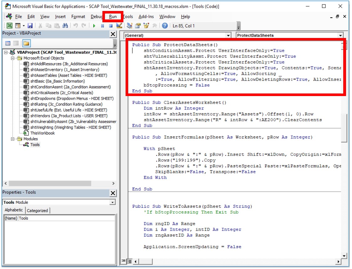
- Protect all sheets by clicking “Run” for the ProtectDataSheets macro in the Macro window as shown above. Note that if password protection is enabled, instructions in this Guide for Tool Managers should be updated accordingly.
Modifying Asset Categories and Types
Overview
You can edit either asset categories or asset types:
- Edit asset categories in the “Dropdown Menus – HIDE SHEET” worksheet.
- Edit asset types in the “Asset Tables – HIDE SHEET” worksheet.
DO NOT edit the asset categories without editing the corresponding asset tables:
- Asset tables depend on the names in the asset categories list; changes to the text in the asset categories table will invalidate the dependent dropdown menus in the asset inventory worksheet.
Instructions
Adding or Editing Asset Types
- Adding new or editing existing asset types does not require any changes to other table names or lists.
- Make changes directly to the tables in the “Asset Tables – HIDE SHEET” worksheet
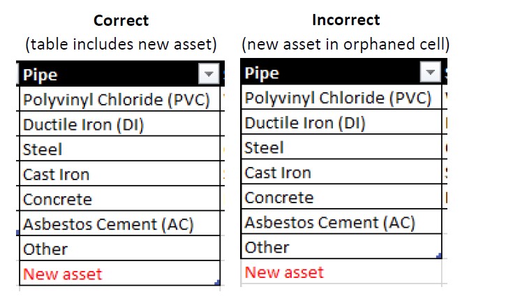
by editing existing asset types or typing new assets at the bottom of each list. To
add the new asset to the table, create an additional row by grabbing and dragging the blue mark in the lower right
corner of the asset column.
Editing Existing Asset Categories
- Make edits directly to the “Asset Category” table in the “Dropdown Menus – HIDE SHEET” worksheet.
- After editing an asset category, navigate to the “Asset Tables – HIDE SHEET” worksheet
and edit the corresponding table headers. Find the asset table with the same header
as the asset category you changed and ensure the text matches exactly.
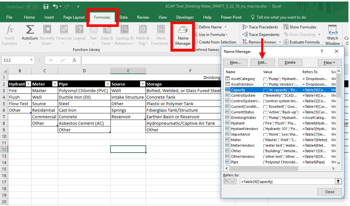
- Edit the corresponding table names using the Excel “Name Manager” tool, which you
can find in the “Formulas” tab, as shown above.
- Find the name in the “Name Manager” list that matches the edited asset category. Click “Edit,” as indicated by the arrow in the screenshot above.
- In the “Edit Name” window that appears (see below), edit the “Name” and “Refers To:” boxes, as indicated by the arrows in the screenshot below. Be sure to make edits that correspond exactly to the new asset category name. (Note, no spaces are allowed in the asset Name field.)
- After you make changes in the “Name Manager” tool, the following items should all match exactly: asset category name (step 1), asset table header (step 2), asset table name (step 3), and the “Name” and “Refers To:” formula (Step 3).
![Screenshot of Edit Name popout window in Excel, with an arrow pointing to the "Name: Hydrant" field and an arrow pointing the "Refers to: =Table6[Hydrant]" field.](/academics/fairmount_las/hugowall/efc/Resources/_images/SCAP-Tool-Managers-Guide-Edit-Name-Manager-Window.jpg)
Adding New Asset Categories
- To add new asset categories, you must create a new named table in the “Asset Tables – HIDE SHEET” worksheet and populate it with asset types for that category.
- Add a new category to the asset category table in the “Dropdown Menus – HIDE SHEET”
worksheet, and make sure to include the new category in the table (similar to step
2 under “Adding or Editing Asset Types” above).
- Create a new table in the “Asset Tables – HIDE SHEET” worksheet. Ensure that the header
matches the new asset category exactly.
- Select the new asset table, click “Format as Table” in the “Home” tab, select any table “Style”, and select “My table has headers,” as shown below and click the “OK” button.
- Select all asset types within the new table (NOT including the table header) and name
the table using the box to the left of the Excel formula bar (see screenshot below).
The name cannot include spaces but must otherwise match the asset category exactly.
- Verify that the table was named correctly in the “Name Manager” window (in the “Formulas”
Tab). Note in the screenshot below that the table name has no spaces but the “Refers
to:” formula does include spaces. The text in the “Refers to:” formula should match
the table header exactly. You may also use “Name Manager” to directly create a new
named table.
![Excel screenshot showing the Name Manager popout window. An arrow is pointing to the "NewAssetCategory" row of the Name column with a note, "No spaces." An arrow is pointing to the "Refers to: =Table29[New Asset Category] field with the note "includes spaces."](/academics/fairmount_las/hugowall/efc/Resources/_images/SCAP-Tool-Managers-Guide-New-Asset-Category-Name-Manager.jpg)
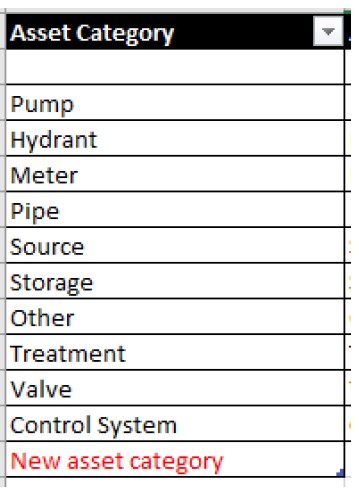
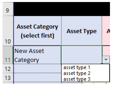
- The new asset category and associated asset types should now appear in the dropdown
menus in the “Asset Inventory” worksheet, as shown below.
- If you add a new asset category and asset types, you must also add the estimated useful life, as described in the next section.
Modifying Estimated Useful Life
Overview
- The tool currently includes useful life estimates that were derived from other vetted sources, including (primarily) the Southwest Environmental Finance Center Asset Inventory Database.
- Note that you may hard-enter custom values for estimated useful life in the “Asset Inventory” worksheet. You should view the default estimates as a starting point from which you can provide more specificity for your assets, if necessary.
- The tool uses the CONCAT function to combine asset category and asset type to automatically populate column A, “For Lookup,” and lists an estimated useful life for each combination of category and type. If you add new asset categories or types, you must also add new rows in the “Est. Useful Life – HIDE SHEET” worksheet.
Instructions
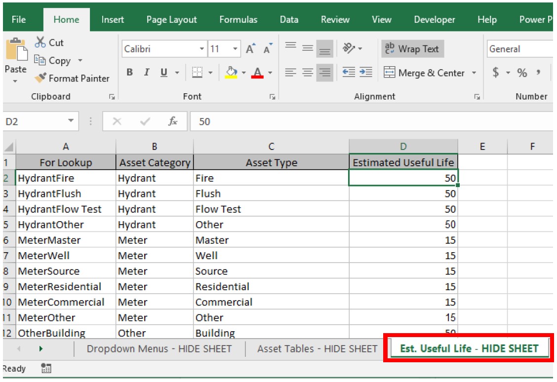
- You can directly edit values for estimated useful life for existing asset types in
the “Est. Useful Life – HIDE SHEET” worksheet, as shown in the screenshot below.
- If you add new asset categories and/or types, you must enter them in the “Est. Useful
Life – HIDE SHEET” worksheet, following the convention shown in that sheet.
- The tool automatically populates “For Lookup” (column A) by combining asset category and asset type using the CONCAT (B#, C#) formula. You should only enter data in columns B, C, and D—"Asset Category,” “Asset Type,” and “Estimated Useful Life,” respectively.
- Any new asset category/type combination must exactly match the category name in the “Dropdown Menus – HIDE SHEET” worksheet and type name in the “Asset Tables – HIDE SHEET” worksheet.
Adjusting Question Weights
Overview
- The tool calculates condition score, consequence of failure, probability of failure, and critical assets and includes weights for each question. You can view and change these weights in the “Weighting Tables – HIDE SHEET” worksheet.
- Each calculation depends on the weights of individual questions and the total maximum score for each question given the defined weights. The tool normalizes the total score for each calculation to the maximum possible value.
- Changes to the weighting for each question will not change the value for each individual answer. For example, an answer of “Excellent” for the asset’s current condition is worth 4 points with a weight of 1. If you change the weight to 2, “Excellent” would be worth 8 points.
Instructions
- Open the “Weighting Tables – HIDE SHEET” worksheet to view weights for each question. The sheet shows the question, other sheets that use the question, and the current weight. It also shows the total maximum score for each calculation. These values automatically calculate and should not be modified.
- Change weights in column C. Weights are multipliers for existing scores and can be any value greater than 0. For example, changing the weight from 1 to 2 will double the value for each response to that question. See the table below for an example of how scores change based on weights for the current conditions question.
- You do not need to make any modifications to individual score calculations once you adjust the weights.
| Current Conditions Responses | Weights | ||
| 1 | 1.5 | 2 | |
| Excellent | 4 | 6 | 8 |
| Good | 3 | 4.5 | 6 |
| Fair | 2 | 3 | 4 |
| Poor | 1 | 1.5 | 2 |
| Very Poor | 0 | 0 | 0 |
Saving and Hiding Tabs
When you have finished editing the hidden tabs and are satisfied the edits work in a manner you expect, you should re-hide the tabs and save the workbook.
- To re-hide previously hidden tabs, right click on each tab you want to hide, and select “Hide.”
- When saving the edited workbook rename the workbook using a file naming convention
that indicates the workbook has been modified, while maintaining a copy of the original
workbook.
Questions? Contact: Brian Bohnsack, Program Manager, brian.bohnsack@wichita.edu, (316) 978-6421